
Making use of the scaling factor command in boundary conditions

This post describes how to use the scaling factor command to adjust time series inputs directly within a boundary condition block in your prefix.grok file. Conceptually, this allows users to scale boundary condition inputs— like fluxes or concentrations— on the fly, without needing to modify large or externally sourced input files. While a straightforward use is unit conversion, we find this command especially useful for quick input calibration during model tuning, allowing users to easily explore how different scaling choices influence model results.
This week’s post will explore HGS’s scaling factor command. Placed inside a boundary condition command, the scaling factor allows the user to scale the associated time series for the HGS run without the need to alter the raw input. Figure 1 is an excerpt from the example model we will be working with in this post and shows how the scaling factor command is to be set up within a boundary condition.

Figure 1: Setup of a scaling factor command
Of course, in the example above, scaling the input by a factor of 2 would have been trivial to do, even without the use of the scaling factor command. However, in most real-world cases where a time series might be made up of thousands of values and/or where the input is read in from a file that might be cumbersome to modify, the scaling factor command is a hassle-free way to scale the input from within the prefix.grok file.
Perhaps the most self-evident use case for the scaling factor is that of unit conversion. This post, however, will showcase another use case – that of on-the-fly input calibration. Because input scaling can be done so quickly via the scaling factor, the user can easily tweak the boundary condition inputs between runs. This can be helpful if the user has reason to suspect that an input might be biased in one way or the other.
Consider this simple model, a variation of the Abdul case.
For this model, we would like to scale the surface flux boundary condition to reproduce the observed output (solid red line) in Figure 2.
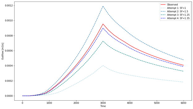
Figure 2: Output hydrographs as a function of scaling factor (SF)
After a few attempts we find that if we use a scaling factor of 1.35, we can get a pretty good approximation of the observed hydrograph.
Now, of course, it is unlikely that any real-world models would simply have a single degree of freedom as in this case, but hopefully this example has given you some inspiration on how to apply the scaling factor command in your own models.